Learning Math with LSTMs and Keras

Updated 5 JUL 2019: Improved the model and added a prediction helper

Updated 19 DEC 2019: Upgraded to TensorFlow 2 and now using tensorflow.keras

Since ancient times, it has been known that machines excel at math while humans are pretty good at detecting cats in pictures. But with the advent of deep learning, the boundaries have started to blur…

Today we want to teach the machines to do math - again! But instead of feeding them with optimized, known representations of numbers and calling hard-wired operations on them, we will feed in strings representing math formulas along with strings representing their results, character by character, and have the machine figure out how to interpret them and arrive at the results on its own.

The resulting model is much more human: Not all results are exact, but they are close. It’s more of an approximation than an exact calculation. As a 100% human myself, I surely can relate to almost-correct math, if anything.

Today’s post will be much more practical than usual, so if you want to build this at home, get your long-neglected Pythons out of their cages! You can find the complete code with lots of improvements here.

NEW: Just try the complete project here in Google Colab!

Recurrent Neural Networks and Long-Short-Term-Memory

As in my previous post, we’re going to use Recurrent Neural Networks, or RNN for short. More specifically, a kind of RNN known under the fancy name of Long-Short-Term-Memory, or LSTM. If you need a primer on these, I can recommend Christopher Olah’s “Understanding LSTMs” and again Andrej Karpathy’s “The Unreasonable Effectiveness of Recurrent Neural Networks”. But to summarize: RNNs are essentially building blocks of Neural Networks that not only look at the current input, but also remember the input before. LSTMs especially have a complex memory mechanism that can learn which parts of the data are important to remember, which can be ignored, and which can be forgotten.

Sequence to Sequence Learning

Sequence to sequence learning deals with problems in which a source sequence of inputs has to be mapped to a target sequence of outputs where each output is not necessarily directly dependent on a single input. The classical example is translation. How do you learn that a Chinese input phrase “他现在已经在路上了。” equals “She is on her way.” in English?

Even with RNNs it’s not directly obvious how to do this. Well, it wasn’t until Google published their paper “Sequence to Sequence Learning with Neural Networks” (Seq2Seq) in 2014. The idea is to train a joint encoder-decoder model. First, an encoder based on RNNs learns an abstract representation. Then a decoder also based on RNNs learns to decode it to another language, generating a new sequence from the encoding as output.

Bidirectional RNNs

It turns out RNNs work much better if we let them look into the future as well. For this purpose, so-called bi-directional RNNs were invented. Each bi-directional RNN consists of two RNNs: One that looks at the sequence from start to end, and one that looks at it in reverse. At each part of the sequence we thus have information about what came before and what will come after. That way, a RNNs can better learn about the context of each segment.

The Setup

For most problems, data is hard to come by. Labeled data even more so. But math equations are cheap: They can be easily generated, and Python gives us their result simply by calling eval(equation_string). Starting with simple addition of small, natural numbers, we can easily generate a lot of equations along with their results and train a Seq2Seq model on it.

For example, a typical datapoint for addition could look like this:

input: '31 + 87'
output: '118'

Since we’re learning on just a fraction of all possible formulas, the model can’t just learn the results by heart. Instead, in order to generalize to all other equations, it really needs to “understand” what addition “means”. This could include, among others:

• An equation consists of numbers and operations
• Two numbers are added up digit-by-digit
• If two digits add up to a value higher than 9, they carry over to the next
• Commutativity: a + b = b + a
• Adding zero does not actually do anything: a + 0 = a
• etc.

And this just for additions! If we add more operations, or mix them, the network needs to grog even more rules like this.

Setting up your Environment

If you’re doing this from scratch, you will want to work in a new virtualenv. I also recommend using Python 3, because it’s really time we got over Python 2… If you don’t know how virtualenv works, I really recommend looking into them. You can find a short tutorial here. To get a virtualenv with Python 3, try virtualenv -p python3 venv.

Once your virtualenv is activated, install these requirements:

pip install numpy tensorflow

If you run into trouble with Tensorflow, follow their guide.

Great! You can paste the code below into a Python shell, or store it in a file, it’s up to you.

Generating Math Formulas as Strings

For now, let’s build some equations! We’re going to go real simple here and just work with easy-peasy addition of two natural numbers. Once we get that to work, we can build more funky stuff later on. See the full code to find out how to build more complex equations.

To make sure we build each possible equation only once, we’re going to use a generator. With the handy itertools Python standard package, we can generate all possible permutations of two numbers and then create a formula for each pair. Here’s our basic code. Note that I’m referencing some global variables (IN ALL CAPS), we will define them later.

import itertools
import random

def generate_equations(shuffle=True, max_count=None):
    """
    Generates all possible math equations given the global configuration.
    If max_count is given, returns that many at most. If shuffle is True,
    the equation will be generated in random order.
    """
    # Generate all possible unique sets of numbers
    number_permutations = itertools.permutations(
        range(MIN_NUMBER, MAX_NUMBER + 1), 2
    )

    # Shuffle if required. The downside is we need to convert to list first
    if shuffle:
        number_permutations = list(number_permutations)
        random.shuffle(number_permutations)

    # If a max_count is given, use itertools to only look at that many items
    if max_count is not None:
        number_permutations = itertools.islice(number_permutations, max_count)

    # Build an equation string for each and yield to caller
    for x, y in number_permutations:
        yield '{} + {}'.format(x, y)

Assuming global config values MIN_NUMBER = 0 and MAX_NUMBER = 999, this code will generate us equations like these:

'89 + 7'
'316 + 189'
'240 + 935'

For any of these equation strings, we can easily get the result in Python using eval(equation).

That was easy, right?

Encoding Strings for Neural Networks

Remember we want to look at the strings as sequences. The RNN will not see the input string as a whole, but one character after the other. It will then have to learn to remember the important parts in its internal state. That means we need to convert each input and output string into vectors first. Let’s also add an “end” character to each sequence so the neural network can learn when a sequence is finished. I’m using the (invisible) ‘\0’ character here.

We do this by encoding each character as a one-hot vector. Each string is then simply a matrix of these character-vectors. The way we encode is quite arbitrary, as long as we decode it the same way later on. Here’s some code I used for this:

import numpy as np

CHARS = [str(n) for n in range(10)] + ['+', ' ', '\0']
CHAR_TO_INDEX = {i: c for c, i in enumerate(CHARS)}
INDEX_TO_CHAR = {c: i for c, i in enumerate(CHARS)}

def one_hot_to_index(vector):
    if not np.any(vector):
        return -1

    return np.argmax(vector)

def one_hot_to_char(vector):
    index = one_hot_to_index(vector)
    if index == -1:
        return ''

    return INDEX_TO_CHAR[index]

def one_hot_to_string(matrix):
    return ''.join(one_hot_to_char(vector) for vector in matrix)

With these helper functions, it is quite easy to generate the dataset:

def equations_to_x_y(equations, n):
    """
    Given a list of equations, converts them to one-hot vectors to build
    two data matrixes x and y.
    """
    x = np.zeros((n, MAX_EQUATION_LENGTH, N_FEATURES), dtype=np.float32)
    y = np.zeros((n, MAX_RESULT_LENGTH, N_FEATURES), dtype=np.float32)

    # Get the first n_test equations and convert to test vectors
    for i, equation in enumerate(itertools.islice(equations, n)):
        result = str(eval(equation))

        # Pad the result with spaces
        result = ' ' * (MAX_RESULT_LENGTH - 1 - len(result)) + result

        # We end each sequence in a sequence-end-character:
        equation += '\0'
        result += '\0'

        for t, char in enumerate(equation):
            x[i, t, CHAR_TO_INDEX[char]] = 1

        for t, char in enumerate(result):
            y[i, t, CHAR_TO_INDEX[char]] = 1

    return x, y


def build_dataset():
    """
    Generates equations based on global config, splits them into train and test
    sets, and returns (x_test, y_test, x_train, y_train).
    """
    generator = generate_equations(max_count=N_EXAMPLES)

    # Split into training and test set based on SPLIT:
    n_test = round(SPLIT * N_EXAMPLES)
    n_train = N_EXAMPLES - n_test

    x_test, y_test = equations_to_x_y(generator, n_test)
    x_train, y_train = equations_to_x_y(generator, n_train)

    return x_test, y_test, x_train, y_train

And later to print out some examples along with their targets:

from __future__ import print_function

def print_example_predictions(count, model, x_test, y_test):
    """
    Print some example predictions along with their target from the test set.
    """
    print('Examples:')

    # Pick some random indices from the test set
    prediction_indices = np.random.choice(
        x_test.shape[0], size=count, replace=False
    )
    # Get a prediction of each
    predictions = model.predict(x_test[prediction_indices, :])

    for i in range(count):
        print('{} = {}   (expected: {})'.format(
            one_hot_to_string(x_test[prediction_indices[i]]),
            one_hot_to_string(predictions[i]),
            one_hot_to_string(y_test[prediction_indices[i]]),
        ))

It is important to note here that the training data uses a max length for the input and output sequences only for numerical reasons. The model is not limited by that length and could look at or output longer sequences after this training.

Building the Model in Keras

Now let’s build the model. Thanks to Keras, this is quite straightforward.

First, we need to decide what the shape of our inputs is supposed to be. Since it’s a matrix with a one-hot-vector for each position in the equation string, this is simply (MAX_EQUATION_LENGTH, N_FEATURES). We’ll pass that input to a first layer consisting of 20 (bidirectional) LSTM cells. Each will look at the input, character by character, and output a single value. All these values together are called our embedding or input representation. Essentially, it’s a vector of values that describe our input sequence.

There are several ways to build a Seq2Seq model. Essentially, you want each timestep in the decoder to have access to both the embedding vector and its own output at the previous timestep. To make this possible, we use RepeatVector to feed the decoder network with the representation in each time step. For a more detailed discussion about Seq2Seq models in Keras, see here.

So after we repeat the encoded vector n times with n being the (maximum) length of our output sequences, we run this repeat-sequence through the decoder: A (bidirectional) LSTM layer that will output sequences of vectors. Finally, we want to combine each LSTM cell’s output at each point in the sequence to a single output vector. This is done using Keras’ TimeDistributed wrapper around a simple Dense layer.

Since we expect something like a one-hot vector for each output character, we still need to apply softmax as usual in classification problems. This essentially yields us a probability distribution over the character classes.

Either way, here is our code:

from tensorflow import keras

def build_model():
    """
    Builds and returns the model based on the global config.
    """
    input_shape = (MAX_EQUATION_LENGTH, N_FEATURES)

    model = keras.Sequential()

    # Encoder:
    model.add(keras.layers.Bidirectional(keras.layers.LSTM(20), input_shape=input_shape))

    # The RepeatVector-layer repeats the input n times
    model.add(keras.layers.RepeatVector(MAX_RESULT_LENGTH))

    # Decoder:
    model.add(keras.layers.Bidirectional(keras.layers.LSTM(20, return_sequences=True)))

    model.add(keras.layers.TimeDistributed(keras.layers.Dense(N_FEATURES)))
    model.add(keras.layers.Activation('softmax'))

    model.compile(
        loss='categorical_crossentropy',
        optimizer=keras.optimizers.Adam(lr=0.01),
        metrics=['accuracy'],
    )

    return model

Training

Training is easy. We just call the fit function of the model, passing handy callbacks like the ModelCheckpoint, which stores the best model after each epoch. Here’s the main function of our code:

def main():
    # Fix the random seed to get a consistent dataset
    random.seed(RANDOM_SEED)

    x_test, y_test, x_train, y_train = build_dataset()

    model = build_model()

    model.summary()
    print()

    # Let's print some predictions now to get a feeling for the equations
    print()
    print_example_predictions(5, model, x_test, y_test)
    print()

    try:
        model.fit(
            x_train, y_train,
            epochs=EPOCHS,
            batch_size=BATCH_SIZE,
            validation_data=(x_test, y_test),
            callbacks=[
                keras.callbacks.ModelCheckpoint(
                    'model.h5',
                    save_best_only=True,
                ),
            ]
        )
    except KeyboardInterrupt:
        print('\nCaught SIGINT\n')

    # Load weights achieving best val_loss from training:
    model.load_weights('model.h5')

    print_example_predictions(20, model, x_test, y_test)

Finally, we need to fill in some of the global variables we used throughout the code. With equations using two numbers from 0 to 999, there’s 998k possible data points. Let’s use 30k of those for our dataset, and validate on 10% of that, meaning we’ll train on about 2.7% of possible equations and expect it to generalize to the remaining 97.3%. That may sound impressive, but Deep Learning is actually used to facing much more dire odds.

Here’s my complete config:

MIN_NUMBER = 0
MAX_NUMBER = 999

MAX_N_EXAMPLES = (MAX_NUMBER - MIN_NUMBER) ** 2
N_EXAMPLES = 30000
N_FEATURES = len(CHARS)
MAX_NUMBER_LENGTH_LEFT_SIDE = len(str(MAX_NUMBER))
MAX_NUMBER_LENGTH_RIGHT_SIDE = MAX_NUMBER_LENGTH_LEFT_SIDE + 1
MAX_EQUATION_LENGTH = (MAX_NUMBER_LENGTH_LEFT_SIDE * 2) + 4
MAX_RESULT_LENGTH = MAX_NUMBER_LENGTH_RIGHT_SIDE + 1

SPLIT = .1
EPOCHS = 200
BATCH_SIZE = 256

RANDOM_SEED = 1

Now we can start training. Either call main() from the shell, or store everything in a file training.py and run it via python training.py.

Try out the model

Let’s write a helper to get the result of an equation as calculated by the model:

def predict(model, equation):
    """
    Given a model and an equation string, returns the predicted result.
    """
    x = np.zeros((1, MAX_EQUATION_LENGTH, N_FEATURES), dtype=np.bool)
    equation += '\0'

    for t, char in enumerate(equation):
        x[0, t, CHAR_TO_INDEX[char]] = 1

    predictions = model.predict(x)
    return one_hot_to_string(predictions[0])[:-1]

Try it (just don’t forget the spaces): predict(model, '123 + 321').

Results

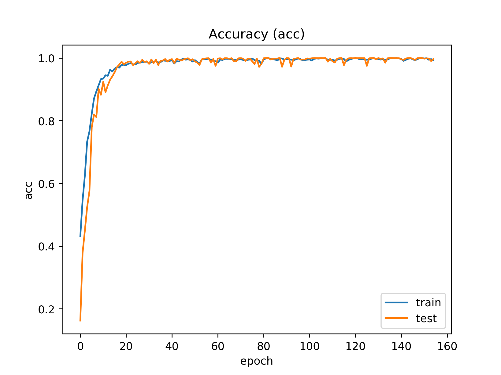
Running the code as it is described here, with some patience I get to a test accuracy of 1.0 on the test set after about 120 epochs. Yes that’s right, it seems we’re making zero mistakes on our test set of 3000 equations. Here’s a graph showing how accuracy developed during training. As you can see, overfitting is not a problem for us. The capacity of the network is just way too small to be learning examples by heart.

That’s great, but running it on some more, unseen example equations, the model still makes the occasional mistake! Why is that? Did our model not generalize to all areas of the problem space?

Analyzing the Mistakes

Let’s look at some of the examples where the model failed to give the right answer. I tried 20k new equations, and out of those, only 10 were incorrect, for example:

47 + 58   = 115  (should have been 105)
94 + 909  = 1903 (should have been 1003)
2 + 7     = 19   (should have been 9)
989 + 811 = 1890 (should have been 1800)
22 + 78   =  00  (should have been 100)

We notice:

1. Most, but not all errors are in the space of smaller numbers, i.e. where at least one number is less than 100.
2. All errors seem to be in one single digit only, while the rest of the digits are correct.

Error #1 is easy to understand: In the lower number range, the rules of addition change a little bit (the first digit no longer counts the 100s). At the same time, this problematic space has seen less training examples than the easier parts. In the whole equation space, there are ~800k points where both numbers have three digits, and only about 80 where both numbers are below 10.

Number two is a bit harder to follow. It seems to be an utterly un-human thing to do. A human would make mistakes in the space of numbers, not in the space of strings. It’s perfectly alright to get the last digit wrong, but to report “1903” instead of “1003” is unacceptable! What happened?

In the case of “1903” vs “1003”, it looks like part of the decoder thought the result would be above 1003, so correctly spit out a “1”, while the next output thought “Nope, definitely below 1000” and output a “9” as in nine-hundred-something. Does each position in the output sequence follow its own stubborn logic, not really caring if the number as a whole makes any sense? This could probably be improved by using a better vector representation or coming up with a better loss function. Or it might be a general weakness in this kind of Seq2Seq model.

Anyway, since our input space has only two factors of variation (the two numbers that go into building the equation), we can plot the equation space in a 2D pane. I went ahead and created a scatter plot with green dots marking correct predictions and red dots marking incorrect ones. Find the code for that here.

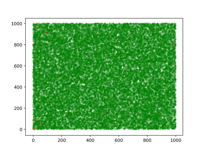
The red dots are hard to see, but they are there!

Further Experiments

There’s lots to do! You can get creative about getting over this lower-number problem. We can also increase the complexity of the equations. I was able to get quite far on ones as complex as 131 + 83 - 744 * 33 (= -24338), but haven’t really gotten it to work with division.

Feel free to pass on hints, ideas for improvement, or your own results in the comments or as issues on my repository.